Quantifying Focus in Computer Vision Use Cases

Updated October 2024

Click here to the demo available in Google Colab

Introduction

Knowing the degree of sharpness or focus in an image is incredibly important when building computer vision systems. In real-world scenarios, cameras often face challenges like vibrations, motion blur, dirty lenses, or improper focus, which result in images that are far from perfectly clear. Any blurring or imperfection in an image can have a major impact on the accuracy of a computer vision model. This is a well-studied issue, whether it affects the training phase of developing a reliable convolutional neural network or when the system is deployed in real-world environments.

Focus Measure Algorithms: An Overview

Quantifying image clarity is critical, and lucky for us, numerous methods have been developed to address this. These techniques range from algorithms that analyze an entire image to those that focus on specific regions or even individual pixels, depending on the use case. The Cheriton School of Computer Science at the University of Waterloo, Canada, has published this excellent paper that compares various focus measures in a clear and accessible way. Rather than summarizing their findings, I’ll take the easy route and recommend reading the paper directly. Then, follow along with my example implementation of the focus measure I’ve found most effective in real-world applications: Brenner’s Focus Measure.

Evaluating Brenner’s Focus Measure Variations

Click here to open in Colab

In this demo, we’ll implement multiple variations of Brenner’s focus measure and then analyze which method is most effective on the GoPro dataset. The full dataset can be found here. We’ll pretend in this scenario that these are images captured by a deployed camera, and our goal is to automatically filter out blurry images.

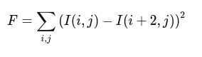
Variation 1: Horizontal Derivative (The Original)

The first variation we’ll implement is the original, which sums the squares of the horizontal first derivative. This is a complicated way to say it measures the difference in brightness between neighboring pixels in the horizontal direction.

def get_brenners_focus_horizontal_derivative(pil_image: Image.Image) -> float:
    """
    Calculate Brenner's focus measure to assess the sharpness of a given image.
    Variation 1 of Brenner's focus measure

    Args:
        pil_image (Image.Image): A PIL Image object to be analyzed.

    Returns:
        float: Brenner's focus measure for the image.
    """
    
    # Ensure the input image is in grayscale mode ('L' mode)
    if pil_image.mode != 'L':
        pil_image = pil_image.convert('L')

    # Convert the PIL image to a NumPy array for efficient processing
    image = np.array(pil_image)

    # Compute the difference between adjacent pixels along the horizontal axis (axis=1)
    diff = np.diff(image, axis=1)

    # Calculate Brenner's focus measure by summing the squares of the differences
    focus_measure = np.sum(diff**2)

    return focus_measure

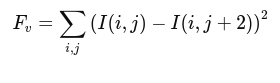
Version 2: Vertical Derivative

The second variation is very similar to the original, however instead of measuring the difference between pixels in the horizontal direction, the derivative is taken in the vertical direction.

def get_brenners_focus_vert_derivative(pil_image: Image.Image) -> float:
    """
    Calculate Brenner's focus measure to assess the sharpness of a given image.
    Variation 2 of Brenner's focus measure
    Args:
        pil_image (Image.Image): A PIL Image object to be analyzed.

    Returns:
        float: Brenner's focus measure for the image.
    """
    
    # Ensure the input image is in grayscale mode ('L' mode)
    if pil_image.mode != 'L':
        pil_image = pil_image.convert('L')

    # Convert the PIL image to a NumPy array for efficient processing
    image = np.array(pil_image)

    # Compute the difference between adjacent pixels along the vertical axis (axis=0)
    diff = np.diff(image, axis=0)

    # Calculate Brenner's focus measure by summing the squares of the differences
    focus_measure = np.sum(diff**2)

    return focus_measure

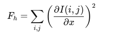
Variation 3: Horizontal Gradient

For the third variation, instead of simply taking difference between adjacent pixels, this variation uses the gradient (rate of change) along the horizontal direction, rather than just the pixel-to-pixel differences as in the original Brenner’s measure. This method is more sophisticated and robust than the original Brenner focus measure because it can better handle subtle changes in intensity and is less sensitive to noise.

def get_brenners_focus_horizontal_gradient(pil_image: Image.Image) -> float:
    """
    Calculate Brenner's focus measure to assess the sharpness of a given image.
    Variation 3 of Brenner's focus measure

    Args:
        pil_image (Image.Image): A PIL Image object to be analyzed.

    Returns:
        float: Brenner's focus measure for the image.
    """
    
    # Ensure the input image is in grayscale mode ('L' mode)
    if pil_image.mode != 'L':
        pil_image = pil_image.convert('L')

    # Convert the PIL image to a NumPy array for efficient processing
    image = np.array(pil_image)

    # Gradient in the horizontal direction
    grad_x = np.gradient(image, axis=1)  

    # Sum of squares of horizontal gradient
    focus_measure = np.sum(grad_x**2)

    return focus_measure

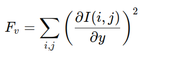
Variation 4: Vertical Gradient

The forth variant we’ll implement is similar to the third variation, however it will instead use the vertical gradient.

def get_brenners_focus_vert_gradient(pil_image: Image.Image) -> float:
    """
    Calculate Brenner's focus measure to assess the sharpness of a given image.
    Variation 4 of Brenner's focus measure

    Args:
        pil_image (Image.Image): A PIL Image object to be analyzed.

    Returns:
        float: Brenner's focus measure for the image.
    """
    
    # Ensure the input image is in grayscale mode ('L' mode)
    if pil_image.mode != 'L':
        pil_image = pil_image.convert('L')

    # Convert the PIL image to a NumPy array for efficient processing
    image = np.array(pil_image)

    # Gradient in the vertical direction
    grad_x = np.gradient(image, axis=0)  

    # Sum of squares of vertical gradient
    focus_measure = np.sum(grad_x**2)

    return focus_measure

Variation 5: Horizontal Derivative (With Color)

This is a variation on the first original equation that computes the horizontal derivative for each color channel (Red, Green, and Blue), and then it averages the focus measures across the three channels. Note that some great next steps would be to call one of the other 3 varations we’ve tested here today instead of the original horizontal derivative variation and evaluate the results.

def get_brenners_focus_color(pil_image: Image.Image) -> float:
    """
    Calculate Brenner's focus measure for a color image by applying the horizontal derivative
    Brenner's focus measure to each color channel (R, G, B) and then averaging the focus measure values.

    Args:
        pil_image (Image.Image): A PIL Image object to be analyzed.

    Returns:
        float: Brenner's focus measure for the color image.
    """
    
    # Convert the PIL image to a NumPy array
    image = np.array(pil_image)
    
    # Split the image into its R, G, B channels
    if image.ndim == 3:  # Check if it's a color image
        red_channel = image[:, :, 0]
        green_channel = image[:, :, 1]
        blue_channel = image[:, :, 2]
    else:
        raise ValueError("Input image must be a color image with 3 channels.")
    
    # Convert the NumPy arrays for each channel back to PIL images so that it's compatible with our previous implementations of brenner's focus measure. 
    red_pil = Image.fromarray(red_channel)
    green_pil = Image.fromarray(green_channel)
    blue_pil = Image.fromarray(blue_channel)

    # Apply the Brenner's focus measure to each channel using get_brenners_focus_horizontal_derivative
    red_focus = get_brenners_focus_horizontal_derivative(red_pil)
    green_focus = get_brenners_focus_horizontal_derivative(green_pil)
    blue_focus = get_brenners_focus_horizontal_derivative(blue_pil)

    # Aggregate the focus measures by averaging them across the channels
    focus_measure = (red_focus + green_focus + blue_focus) / 3

    return focus_measure

Evaluating Brenner’s Variations for the GoPro Dataset

In order to evaluate each focus measure varation’s ability to distinguish between blurry and clear images, lets assume that the larger absolute difference (separation) between the clear set’s mean focus measure and the blurry set’s mean focus measure the better.

In order to do this, for each brenner’s focus measure variation we implemented, we will calculate the mean focus measure for both the clear set of images, and the blury set of images. Then, we’ll find the difference between each set’s focus measure mean. We’ll also plot the focus measure for each image so we can visually verify the results.

If you’re not following along in the colab note book, this evaluation code can be found in demo.ipynb.

Results

Variation 1: Horizontal Derivative (The Original)

Blurry Images - Mean: 10532908.25
Clear Images - Mean: 18553935.046666667
Separation: 8021026.796666667

Version 2: Vertical Derivative

Blurry Images - Mean: 12077206.03
Clear Images - Mean: 20029785.356666666
Separation: 7952579.326666666

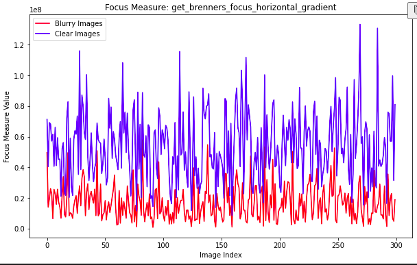
Variation 3: Horizontal Gradient

Blurry Images - Mean: 16788168.4025
Clear Images - Mean: 54070488.63333333
Separation: 37282320.23083334

Variation 4: Vertical Gradient

Blurry Images - Mean: 21482787.395833332
Clear Images - Mean: 55197934.09
Separation: 33715146.694166675

Variation 5: Horizontal Derivative (With Color)

Blurry Images - Mean: 10792328.3
Clear Images - Mean: 18960645.175555553
Separation: 8168316.875555553

Looking at our results, Variation 3: Horizontal Gradient produced the largest absolute difference (separation) between the clear set’s mean focus measure and the blurry set’s mean focus measure the better. This can also be visually verified in the visual produced by our evaluation function.

Threshold Based Filtering Using Focus Measures

Based on the assumption that the larger the absolute difference between the clear set’s mean focus measure and the blurry set’s mean focus measure the better, we’ve found our best and worst variations of brenner’s focus measure.

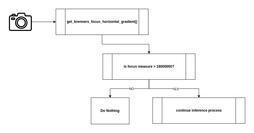
In the introduction I mentioned that for the sake of understanding we were going to pretend in this scenario that these are images captured by a deployed camera, and our goal is to automatically filter out blurry images. We found that our third variant that used the horizontal gradient variation of brenner’s focus measure was best at distinguishing between clear and blurry images. Also, we found that the variant that uses the vertical derivative was the least effective. Now we’re going to evaluate each of these variations by their ability to detect blury images. Imagine our system has a sensor that captures images but before passing each image to inference, a focus measure for that image is calulated. If the image’s focus measure value is sufficient, it will continue on to inference, else, it will be dropped.

Evaluating our best and worst focus measure variations

Lets assume that our use case allows at most a false positive rate of of 3% (clear images incorrectly deemed too blurry). That means for both focus measure variations we’re going to evaluate, we need to select a threshold that at most results in a 3% reduction in clear images. Success will then be measured by the quantity of blurry images filtered out.

For our best variation with a selected threshold of 16810000 we get the following result:

Of 1028, 583 blurry images were dropped successfully (56.71% reduction)
Of 1029, 30 clear images were incorrectly dropped (2.92% reduction)
Precision: 0.95, Recall: 0.57, F1 Score: 0.71

For our worst variation with a selected threshold of 7695000 we get the following result:

Of 1028, 193 blurry images were dropped successfully (18.77% reduction)
Of 1029, 30 clear images were incorrectly dropped (2.92% reduction)
Precision: 0.87, Recall: 0.19, F1 Score: 0.31

Conclusion

Hopefully by now you’ve run all the cells and have been able to successfully recreate the experiment.

In this demo we have:

Loaded a dataset from roboflow
Implemented 5 variations of brenner’s focus measure
Found what is measured to be the best and worst variations for our dataset
Simulated a threshold based filter on our dataset to further compare the effectiveness of these variations

We found that the horizontal gradient based variation of brenner’s focus measure was effective in measuring blur in our dataset and could offer an estimated 56% reduction in blurry images.

Bowen Kruse